Geometric Perspective on Linear Transformations
- What Exactly is a Matrix?
- > Geometric Perspective on Linear Transformations
- System of Linear Equations
- How to rotate a point about the origin
- How to rotate a point about the origin (way 2)
- How to rotate a point about another point
- How to rotate a point about another point (way 2)
In the last post, we discused what linear functions were and how matrices simply represent linear functions. One domain where we often work with linear functions is spatial manipulations. When you want to take a point (or a bunch of points) and sqush, expand, rotate, skew, or translate (move) them, you usually apply a linear function to them. Each component of the transformed point is a linear combination of each component of the input point.
Moving Space
First, we need to think of a spatial transformation as the basis vectors transforming. You start out with some basis vectors, usually <1,0> and <0,1> (called the standard basis vectors), and you move to some other basis vectors. The thing is though, that if your transformation is linear, each of your new basis vectors will be a linear combination of your old basis vectors!
Let’s say that you have the following basis vectors:
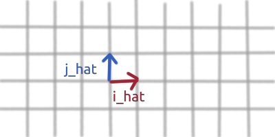
The point <1,1> would be here:
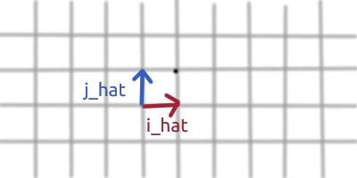
The reason why we know it is there is because the point <1,1,> tells you to go 1 along the i hat and 1 along the j hat.
Now, let’s say that you want to transform this space such that your new i_hat and j_hat are a linear combination of your old i_hat and j_hat. More concretely, let’s say your new_i_hat is 2 * your old_i_hat + 1.5 * your old_j_hat. And let’s say that your new_j_hat is -1 * your old_i_hat + 1 * your old j_hat. Here is what your new i_hat and j_hat would look like, superimposed on your old i_hat and j_hat:

Now let’s put the point <1,1> on these new basis vectors:
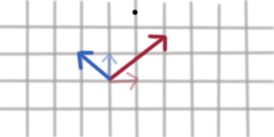
Notice that relative to our new basis vectors point <1,1> is still 1 along the new i hat plus 1 along the new jhat direction. But relative to the old i hat, j hat, the point <1,1> has moved significantly!
Think of it this way. Any point that you are given, the coordinates (or components) of the point specify how much to go along i and j hat. In other words they specify the coeffecients for the linear combinations of the i and j hat vectors that give you the destination of that point.
Our original point was <1,1> (relative to our original basis vectors), our point <1,1> is still 1 along the new i and j hat, but relative to our old basis vectors it is now at <1,2.5>! We can say that we have linearly transformed our point. This linear transformation is entirely encoded in our new basis vectors. We can store this in a matrix by putting our new i hat in the first column and our new j hat in the second column, as follows:
[2   -1]
[1.5  1]
If we think about the rules of matrx vector multiplication (aka vector transformation), we realize that the first component of our output vector (the x component), will have the scaled up sum of the x components of our new basis vectors, while the 2nd component of our output vecotr (the y component) will have the scaled up sum of the y components of our new basis vectors!
Quick note here. Remember the last article? We said that by convention, each linear combination (1 per output component) is on a seperate row of the matrix? We’ve stuck true to that. The first row has the coeffecients for the x output’s linear combination, while the second row has the coeffecients for the y output’s linear combination. Furtheremore, it kind of makes sense that our new x will be a linear combination of the x components of our new basis vectors. Similarly, our new y will be a linear combination of the y components of our new basis vectors.
Mapping the Same Point Between Different Basis Vectors
Imagine a space with many different basis vectors. Each physical point in this space can be described as relative to any of the basis vectors. If you are given the coordinates of a physical point relative to one of the basis vectors, how can you find out what the coordinate of this same physical point is, relative to another basis vector?
You need to know the relationship between the two basis vectors. That is the obvious link. If you know the physical point is described by <1,1> relative to basis vectors i and j, then in order to know what coordinate represents this same physical point relative to basis vectors k and l, you need to know the linear function between these two basis vectors. More concretely, you need to know i and j in terms of k and l!
Summary
In the last article in this series, we learned that matrices represent linear transformations. In this article, we looked at linear transformations geometrically. We can of course still think of a linear transformation as a transformation where each of our output components is a linear combination of each of our input components, however, it can be helpful to take a different (and equally true) perspective. We can think of a linear transformation as our basis vectors transforming. Our new basis vectors are a linear combination of our old basis vectors. Put the linear combination of each new basis vector in a seperate column (not row) of a matrix.