Description
Find Value Function Using Bellman’s Equation Directly
Find Value Function Using Monte-Carlo Methods
Find Value Function Using TD Methods

Description

Just a markov process with an associated “reward” at the end of each arrow!

+----------+                            +----------+
|          |   p = 0.3                  |          |
| state 1  |  ------------------------> | state 2  |
|          |               reward = 1   |          |
+----------+                            +----------+
     |                                              
     |                                  +----------+
     |   p = 0.7                        |          |
     +--------------------------------> | state 3  |
                           reward = 2   |          |
                                        +----------+

Once you add rewards, you can begin to do some reinforcement learning. Once you cross an arrow, you get the reward at the end of that arrow.

The value function of the process tells you how “valuable” a particular state is in the long term. Meaning, that if you start in that state and let the markov reward process (MRP) rip (let-er riiiip!), how much total reward will you collect as you flow through the MRP? If you are in a high value state, then you are likely to end up collecting a lot of reward if you continue from this state.

There are several ways of finding the value function:

Directly: You could directly solve the bellman expectation equations
You could use monte-carlo (MC) methods to run “trials” (“simulations”, “episodes”) in the markov reward process
You could use TD methods to run more “efficient” trials

Find Value Function Using Bellman’s Equation Directly

The equation in words:

The value of a state is the expected return if you start in that state.

In pseudocode (python like):

def value(state):
    expected_return = 0
    for each edge
        expected_return += probability of following that edge * (reward at end of edge + discounted value for state landed in)
    return expected_return

In equation form heh-heh:

$v(s) = \mathbb{E}[G_t | S_t = s]$ $v(s) = \sum_{s\prime} p(s\prime | s) (R(s,s\prime) + v(s\prime))$

Where

$v(s)$ is the value for state $s$
$\sum_{s\prime}$ is “(sum) for each state $s\prime$ that can be reached directly from state $s$ ”
$p(s\prime \| s)$ is the probability of coming to state $s\prime$ from $s$
$R(s,s\prime)$ is the reward you get for going from state $s$ to $s\prime$
$v(s\prime)$ is the value for state $s\prime$

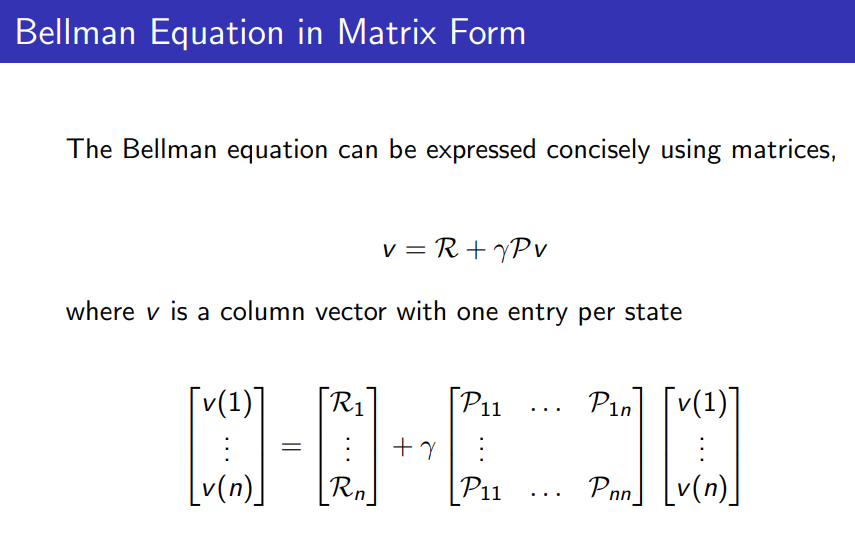
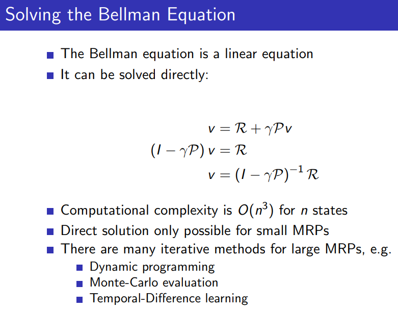
There is one bellman expectation equation for each state. There is vector-matrix form of the bellman’s expectation equation so that you can solve the system of equations easier (by doing matrix inversion).

These two slides from David Silver’s RL lectures show the matrix form of the equation: david silver RL slide 1

But, you can only use this method (directly solving bellman’s expectation equations to find value function) if you know the dynamics of the MRP. Knowing the dynamics means knowing things like “if I’m in state s and I take action a, what is the probability that I’ll end up in state s_prime? What about rewards? What rewards might I end up with and what are the probabilities of each?”. A lot of the times, you do not know the dynamics, but you can run simulations (or the real thing) and still figure out the value function! Also, even if you know the dynamics, it is often easier (because calculating probabilities is sometimes hard) and more efficient to just run simulations, and learn the value function from the simulations.

Find Value Function Using Monte-Carlo Methods

The basic idea: run a bunch of episodes through your markov reward process. For the episodes that you encounter your state of interest (the state whose value you’re interested in calculating), keep track of the total reward you collect after you see the state of interest (until the very end). So in other words, how much reward was accumulated after you saw your state of interest till the end. We’ll call this the “responsible reward”. Average a bunch of “responsible rewards” for your state (each seen at a different episode), which should give you an idea of the “value” of your state, on average, according to your observed episodes. If you run enough episodes, this should converge to the actual value of the state (as would be predicted by the bellman expectation equation, if you knew the dynamics).

The above method ignores subsequent visits to the same state (in the same episode). A little modification to the above monte-carlo method (called “every-visit monte-carlo”) states that you should not ignore subsequent visits, but that every time you visit your state of interest, you should take the “responsible reward” (from this state till the end) and average it into your average for the state so far.

You’ll usually see these algorithms working backwards (they start from the last state and work to the first), because it’s more efficient that way.

Monte-carlo methods require episodic tasks. TD Methods do not (and they are more efficient).

Find Value Function Using TD Methods

Basic idea: Don’t wait till the very end of the episode to update your guess of the value for the state.

In TD n=0, you will update value for state s as soon as you experience state s_prime. Move your guess for state s’s value a little closer to: (reward for coming to state s_prime + value of state s_prime). In TD n = 1 will wait one more state, so you will sum two concrete rewards to the value of the third state. TD n = 2 sums 3 concrete rewards plus the value of the fourth state. I think you see the pattern.

Hell, you can even do several n’s, and then “weighted” average them (giving less and less weight to higher ns). This is called TD lambda. Lambda tells you how much to decay the weight for each n. A lambda of 0 is equivalent to TD n = 0, because it will give all higher ns a weight of 0. A lambda of 1 is equivalent to MC because it gives all ns equal weight. If you give all ns equal weight, you are basically doing MC.